Designing ophthalmology services - Part 1: How do we address the queues in a clinic?
By Kate Silvester

This first of a three-part series shows how systems engineering can be used to correctly diagnose and address the causes of delays in a clinic. The second article, which will be featured in the April/May 2020 issue, describes how to design a more productive system that meets the new and follow-up demand.

The Systems Engineering Approach

Ophthalmology is a complex ‘repair and overhaul’ system in which there is a high variety of patients and clinical conditions that share resources. Many patients, especially those requiring follow-up, ‘loop back’ through these resources as indicated in Figure 1 below.

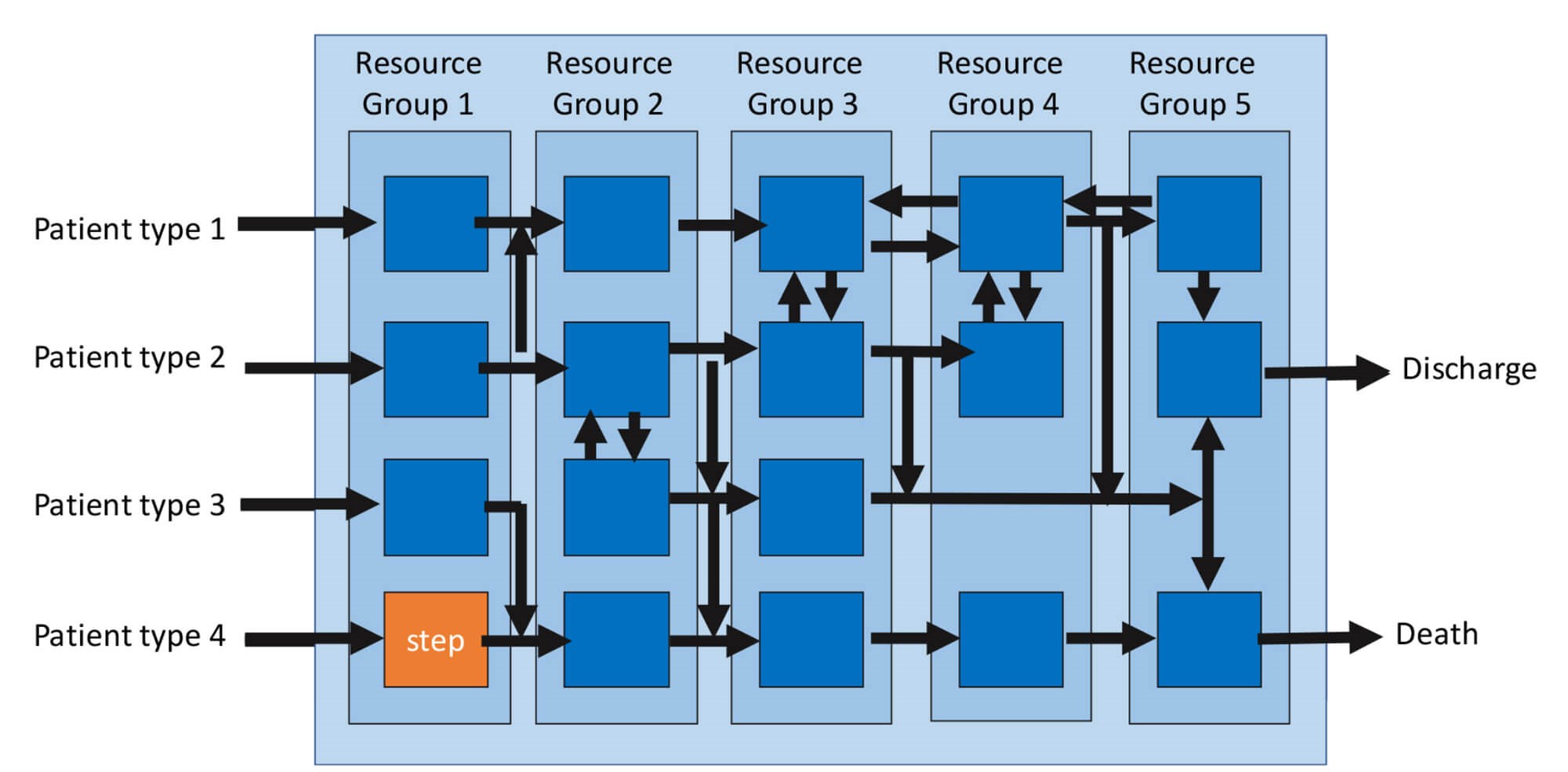
Figure 1: The two views of a complex system.

Principle 1: There are two views of a system

1. The first is from the resource’s perspective (the vertical stages):
   • In this case, we will consider the resource cost as the time that the resource is scheduled (and therefore paid) to be available, e.g. four hours = 240 minutes x cost/unit time.
2. The second view is from the patient’s perspective (the horizontal streams):
   • The effectiveness i.e. the quality or yield: Did the patients get what they requested? i.e. the correct diagnosis (“What’s wrong with me?”), prognosis (“When will I get better?”) and a plan (“How do I get better and stay well?”) Every review offers the resource and patient an opportunity to assess the yield from the previous intervention, and yet this feedback loop in our system is intermittent (occasional audit) or entirely lacking.
   • The time the patient spends waiting to attend our services. Systems Engineering is a well-established discipline for ensuring that such complex systems are designed to be productive, i.e. cost effective [1]. The starting point is to consider the flow through the simplest of systems; one resource (a step) as indicated by the orange box, e.g. one nurse and a Snellen chart.

Principle 2: There are four measures of flow through a system

• Flow in: Demand = requests / time
• Flow out: Activity = requests met / time
• WIP (Work in Progress): number of patients in the system at a point in time
• Lead-time: the time from request being made to request being met

If the average queue or work-in-progress (WIP) is stable over time, then what is flowing in must be flowing out and the average WIP /average flow = average lead-time in the system. Little’s law [2] describes this relationship and given any two parameters for a stable system, we can predict the third.

WIP is the most sensitive indicator of changes in flow as it is the cumulative difference between the demand and the activity. If the WIP is not stable over time, then there must be a mismatch between the demand and activity. This could be caused by a change in a scheduling policy that is ‘holding patients up’.

Principle 3: Measuring the workload on a step.

To understand the workload being placed on a resource, we need to measure the time it takes to process patients. The cycle-time is the time from when the resource starts work on one patient to when the same resource is ready to start the next patient. The cycle-time is the touch-time (time with the patient) plus the changeover-time (which includes the admin tasks required before calling in the next patient).

For example, if 20 patients are scheduled for an elective, four-hour clinic and the average cycle-time of the nurse is five minutes / patient, then the workload is =20x5=100 minutes to be scheduled over the 240-minute period. If the patients are booked in faster than one patient every five minutes then a growing queue will form.

Queues cause delays and overburden resources thereby increasing the stress, increasing the risk of error and reducing the yield (the % of patients seen who got the right care). They also increase costs as more resource-time is required to manage the queues and more capital resource is needed to store the queues.
Now let us consider the next level of complexity: A sequence of steps as in a clinic.

Principle 4: Every system has a constraint.

In a sequential process, one of the steps will have the longest cycle-time and will be the flow constraint. There is no point of any upstream resource working faster than the constraint since this will only create a queue at the constraint [3]. Ideally, we want the most value-adding and most expensive resource / min to be at the constraint step as this will improve the productivity of the whole system.

Case Study: Diagnosing the cause of a queue in a general retinal clinic

Caveat: The data for this clinic were collected seven years ago and since then optical coherence tomography (OCT) has been introduced to retinal clinics.

The purpose of this paper is to demonstrate the engineering principles in a relatively simple system with no case mix variation, i.e. one process type.

The issues with this clinic were that:

1. The waiting room filled up so that the elderly patients and their carers had to stand
2. The clinic regularly over-ran
3. The staff and patients were stressed
4. The nurse and optometrist were ‘rushed of their feet’ and resented having to stay on late to clear up
5. The ophthalmologist was frustrated as he often found himself with nothing to do and was then rushed at the end of the clinic.

Diagnosing the cause of the queues

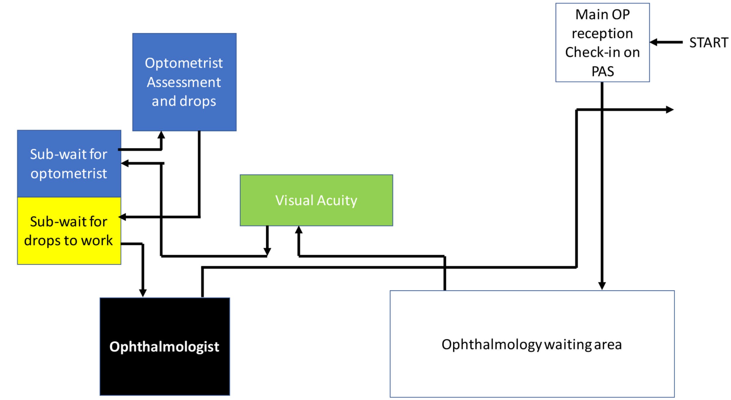
Figure 2: The flow of patients through the clinic.

Patients arrived and were checked-in at the main out-patient reception on the hospital’s patient administration system (PAS). They waited in the main ophthalmology waiting area and were then called by the nurse for their visual acuities (VA). They waited again for assessment by an optometrist in the first of two consulting rooms who also gave the patients drops to dilate their pupil(s). They then waited outside the second consulting room for the drops to work before their consultation with the ophthalmologist.

Since the PAS and the electronic clinical record were separate systems and the patients did not ‘check-out’ on PAS, the following data were collected manually. The main receptionist handed each patient a paper slip onto which they recorded their appointment time and arrival time. The clinical staff then recorded their start and finish times with each patient. The ophthalmologist recorded both the touch-time and the subsequent admin-time with each patient in order to capture his total workload. These slips were collected at the end of the clinic and entered into Excel as shown in Table 1.

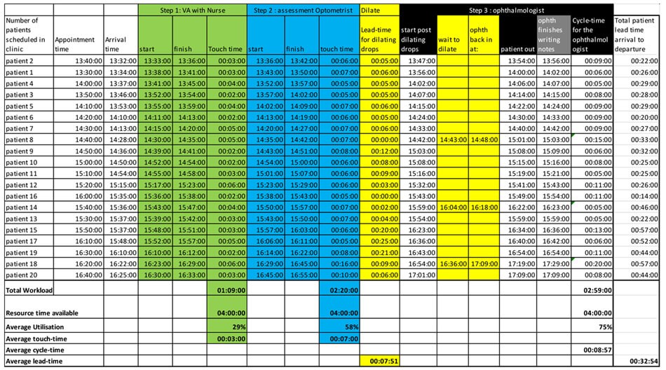
Table 1: Start and finish times at each resource (in HH:MM:SS format) for 20 patients.

Table 1 illustrates the detailed data set of events for one clinic. How do we make sense of so much data?
First, we can look at the lead-times (arrival to departure) for patients (Figure 3). Since the clinic operated a ‘first come first served’ policy, the patients’ lead-times were plotted in arrival order.

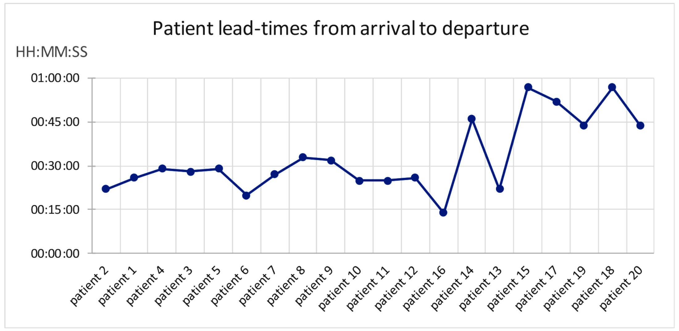
Figure 3: Consecutive patients’ lead-times through a general retinal follow-up clinic.

From the average times the patients spend at each resource (three. Seven, eight and nine minutes in Table 1) we would expect the patient to spend an average of 27 minutes in the clinic.

Figure 3 shows that although the average lead-time for the clinic might be reported as 32 minutes, the first 13 patients spent less than 30 minutes in the clinic, but then the system ‘flipped’ and then six patients took nearly an hour. If there was not enough resource time to meet workload, then we would expect the lead-times to steadily increase as the clinic progressed.

So, this pattern suggests that something else is going on.

Making the system behaviour visible

A Gantt chart [4] turns the mass of data in Table 1 into a picture that exposes the variation in the system.

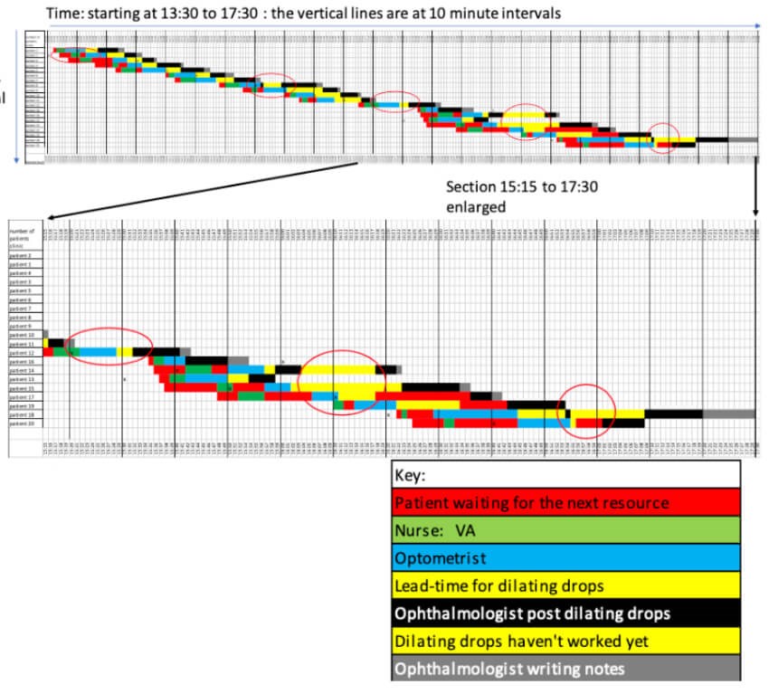
Figure 4: The Gantt chart.

Time is recorded horizontally and the patients (in their arrival order) are recorded vertically. Each step in a patient’s process is represented as a horizontal bar and the time with each resource is colour coded as in the key. Red bars show when a patient is waiting for a resource and the red circles show when the ophthalmologist is waiting for a patient.

A Gantt chart is usually an eye-opener for all the stakeholders as normally only the patients experience the flow through the system.

1. The data show that most patients arrived early for their appointment and wait for the first resource.
2. The red bars show that the patients did wait a short time (red) for the optometrist (blue).
3. The ophthalmologist (black) had to wait 16 minutes (first red circle) until the first patient had dilated sufficiently to make a diagnosis, prognosis and plan.
4. The system runs ‘smoothly’ (rate in = rate out) until Patient 8, who was not sufficiently dilated for the ophthalmologist to proceed. The patient (yellow bar) and ophthalmologist waited (second red circle).
5. The system continued to run smoothly until Patient 12 when the ophthalmologist ran out of work at 15:20 and had to wait for the optometrist and the dilating drops to work (third red circle).
   The ‘tipping’ point for this clinic is reflected at the point when the WIP (the number of patients in the clinic) increases from three to five (Figure 4) and the increase in the patients’ lead-times (Figure 3). To see what is going on, the subsequent section of the Gantt chart has been enlarged (Figure 4).
6. Patient 13 was seven minutes late, but Patients 14 and 16 are early. Despite being late, Patient 13 is dilated before Patient 14 and then the ophthalmologist has to interrupt the consultation with Patient 14 to wait for the drops to take effect, but Patient 15 isn’t ready either (third circle).
7. Now there is a ‘pile-up’ of four patients who, despite arriving early, the optometrist could not process any quickly enough.
8. We now have the worst of all worlds: Patients waiting in the wrong order and an ‘idle’, expensive resource, the ophthalmologist, waiting too (fourth and fifth red circles),
9. In a desperate attempt to progress the patients and finish on time, the nurse, optometrist and ophthalmologist were shuffling elderly patients (who can’t see very well) in and out of the two rooms. The system was now fraught with potential errors and harm.

It would be easy to blame the late patient for the ‘pile-up’ at 15:35 and reduce the appointment interval and / or add-in an extra patient in the hope that a queue of patients in front of the ophthalmologist would buffer him from any patients who are late (or DNAs) in the future.

Rather than leap to a ‘solution’, we first need to be sure that there isn’t another underlying cause for the sudden appearance of the queue.

Differential diagnosis

1. Is there a resource time constraint? 
   • Scheduled resource time capacity 13:30 to 17:30 = 240 minutes.
   • Scheduled demand = 20 patients.
   • Appointment interval, one patient every 10 minutes from 13:30 to 16:50. Summing the touch-times for the nurse and optometrist, their average utilisations are 28% and 58% respectively. Summing the ophthalmologist’s cycle-times, the average utilisation of the ophthalmologist (our most expensive resource) is 75%.
   • None of the staff were over-loaded, so there was no resource time constraint.
   • The diagnosis was, therefore, a policy constraint.
2. Where is the policy constraint? The average touch-times for the nurse and optometrist are 0:03:24 and 00:07:00 respectively. When the optometrist is not waiting for a patient, we can calculate her admin time as an average of 00:01:00 giving her cycle time as an average of 00:08:00. So, the ophthalmologist, with a cycle time of 00:08:59, is still the constraint and therefore should not wait for work. (It would also be tempting to improve the efficiency of the clinic by adding the nurse’s VA work to the optometrist since her utilisation is only 25% and the optometrist’s is 55%. However, we can now see the error of adding the VA (or future OCT) work to the optometrist. This would result in the optometrist’s cycle-time equal to 00:11:30, making her the constraint and unable to keep pace with the ophthalmologist, the most expensive resource. We might save the cost of a nurse, but we will reduce the productivity of the clinic as we will see fewer patients in 240 minutes, make the delays for patients worse and stress the two remining staff with a growing queue).

Underloading the clinic

In this case the appointment interval is 00:10:00 so the patients are not being scheduled into the clinic fast enough to meet the rate at the constraint (00:08:59). We would expect the ophthalmologist to run out of work, as he does at Patient 8, who was not sufficiently dilated when he was ready.

Making the clinic resilient to variation

We need to buffer the clinic resources to deal with the variation in demand (patients arriving late or DNA) and cycle-times including the dilating time. We could do this by:

a) Scheduling the patients in at an average of nine minutes. 

• In this case the scheduled demand is finite (20 patients) and the ophthalmologist will be able to catch-up after the last patient arrives if there is a run of patients with longer than average cycle-times.

b) Having a buffer of two patients, rather than one, in front of constraint.

• This will help protect the ophthalmologist from a run of patients with shorter than average cycle-times and ensure that at least one patient’s pupils are dilated before they see the ophthalmologist.

A future state Gantt chart based on the average cycle times suggests that we can achieve this new design with 20 patients starting at 13:30 and subsequent appointment intervals of 5, 10, 10, 10, 10, 10, 10, 5, 10, 5, 10, 10, 10, 10, 10, 10, 10, 10 and 5 minutes. The 20th patient would finish at 16:30.

Provided we keep the ‘first in first out’ policy, could we schedule a further three patients in at 16:15, 16:25, 16:35 and finish before 17:15, giving adequate time for a patient arriving late and letting the staff clear up and get away before 17:30?

However, a stock and flow chart in Excel that accounts for the variations in cycle-times shows that, provided all patients arrive on time, only 22 patients can be scheduled into the clinic and finish reliably before 17:30 (9/10 clinics).

This would mean that we would solve all the patients’ and staff issues and increase the activity by 10% for no further increase in cost other than an extra chair outside the consultant’s room! We would have to revisit this design when OCT is introduced.

Conclusion

This case study shows that even single-stream ophthalmology clinics with minimal case-mix variation are complex systems and their behaviour is non-linear and counter-intuitive. Other teams have applied system engineering principles [5] to diagnose and improve the flow through more complex clinics [6,7,8] and the data collection can be automated [9]. All have discovered that it is vital to diagnose correctly the constraints specific to their system before making changes.

The next paper considers how, once we have discovered the cycle-time for the resources in a system, we can calculate the number of new and follow-up appointment slots required to ensure all patients receive their care on time.

TAKE HOME MESSAGE

• Ophthalmology clinics are complex systems that behave in non-linear and counter-intuitive ways.

• Simple and ‘obvious’ solutions to delays can make performance worse.

• To deliver the benefits of clinical innovation, we need to understand our systems of care, diagnose the constraints and engineer systems that are resilient to expected variation.

References

1. Dodds Simon: Three wins. Kingsham Press: Chichester; 2006.
2. Little JDC. A Proof for the Queuing Formula: L = λW. Operations Research 1961;9(3):383-7.
3. Goldratt EM: Theory of Constraints. The North River Press; 1999.
4. Gantt H (1861–1919), who designed such a chart around the years 1910–1915. Source:
https://en.wikipedia.org/
wiki/Gantt_chart
5. Dodds Simon. Healthcare system engineering course. Online:
https://www.saasoft.co.uk/
index.php
6. Dowdall M: 6M Design® in Our Hands - Improving Paediatric Ophthalmology In-Clinic Flow. Journal of Improvement Science 2018;53:1-17.
7. Roberts H, Silvester K. Finding the Constraints in an Ophthalmology Clinic. Journal of Improvement Science 2017;45:1-21.
8. Adams A. Diagnosing Flow Constraints in a Fast Track Glaucoma Clinic. Journal of Improvement Science 2019;61:1-10.
9. Silvester KM, Patel J. Introducing eleGANTT®: An automated tool for real-time diagnosis of the constraints in ophthalmology clinics. Journal of Improvement Science 2019;54:1-15.

Declaration of competing interests: None declared.

Acknowledgement:
The author would like to thank the team at George Elliot Hospital, Nuneaton for their data.

Part 2 of this series can be found here
Part 3 of this series can be found here

COMMENTS ARE WELCOME